Building a Search Engine That Actually Works:
Optimizing RAG Retrieval for Technical Documents
One of the most grounding projects I’ve built during my journey of learning AI/ML has been building a materials reference system — a local RAG application that serves a corpus of Materials Science handbooks covering essentially every materials topic under the sun. I am constantly going back to these handbooks to pull references and expand my knowledge when something specific comes up. The system I built has three roles: a semantic search engine for the corpus, an agentic retrieval pipeline, and topic-based browsing. While the agentic capabilities of this system are what I’m most excited about, having searchability of this corpus was something that would provide me with immediate value.
This post covers the first role of the system: making search actually work. The system design was focused first and foremost to be a local tool for myself, but in the near future it’ll get stood up in the cloud.
When I first built the retrieval pipeline (with the help of Claude), it was broken in ways I couldn’t immediately explain. Queries that should have returned corrosion properties for specific alloys returned results about the correct alloy, but nothing about corrosion. Or, the results would prominently feature corrosion, but for a completely different metal (e.g. steel instead of brass). I knew something major was wrong, but I didn’t know what it was or how to measure it.
Measuring the Baseline
Instead of blindly telling Claude “This is not working, fix it”, I needed to understand how the tool actually functioned. I fell back to my experience in process engineering, as they say in Lean Six Sigma, that which you do not measure cannot be improved. So, I needed to know what I was starting with, how are search & RAG systems measured?
The primary metric I used is NDCG@5 - Normalized Discounted Cumulative Gain at rank 5 - which is a mouthful, but it essentially means you reward highly relevant results that appear early in the ranked list and you penalize results that appear late. A score of 1.0 is perfect; 0 means nothing relevant appeared.
The way it gets measured is straightforward once you break it apart. You need a set of test queries based on the actual data in the corpus (using a testing subset). For each test query I labeled specific chunks in the test set that are actually relevant and and rated them on how relevant they are (2 for a direct hit, 1 for related context, 0 for irrelevant). When the search returns its top 5, each result earns points based on its relevance label, but those points get discounted the further down the list they sit — a relevant chunk at position 1 is worth its full value, position 2 is worth a bit less, position 5 quite a bit less. Sum those discounted scores, then divide by the score you’d get if the results were ranked perfectly. That ratio is the “normalized” part, and it’s what makes 1.0 the ceiling regardless of how many relevant chunks exist for a given query.
In practice, that means a score of 0.8 isn’t “80% correct” in any intuitive sense — it means the ranking is mostly getting the right stuff near the top, with some shuffling or a near-miss in the mix. For a technical reference system where I want a specific data point in the top few results, that ranking sensitivity is exactly what I need. I also tracked Precision@5 (fraction of the top 5 results that are relevant) and Fidelity (the fraction of all known-relevant chunks that appear anywhere in the retrieved set - a recall diagnostic).
For this testing, I subsetted the corpus and pulled 16 specific documents. Then, I created a labeled test set of 40 queries covering six categories: specific alloy property lookup, corrosion behavior, alloy designation/composition, process and heat treatment, comparative queries, and cross-property/application questions. All of the queries were ranked. If I had done this by hand it would’ve taken me forever, so I pulled in Claude to help. I needed to eliminate any possibility of hallucinations or misrepresentations of the data in the test set, so I had Claude provide specific citations for each query which I then verified and personally rated. I could’ve taken some shortcuts here, but I wanted to make sure this test set was rock solid.
The baseline system used SQLite FTS5 full-text search combined with sentence-transformer semantic embeddings, merged via Reciprocal Rank Fusion (RRF). The results were sobering:
| Metric | Baseline |
|---|---|
| NDCG@5 | 0.101 |
| P@5 (any relevant) | 0.080 |
| P@5 (highly relevant) | 0.080 |
| Fidelity | 0.041 |
A fidelity of 0.041 means the system was recovering less than 5% of all known-relevant chunks. Relevant content existed in the index. It was just never returned. Final verdict, the first pass build of this system was pretty much garbage.
Diagnosing Five Root Causes
Working through the code, I found five big problems. Each of these failures is a lesson learned, and on the next system I build not one of them will happen again.
Silent embedding truncation was the most damaging. The production system used all-MiniLM-L6-v2, a model with a 256-token input limit (roughly 190 words). Chunks were configured at 512 words. The final ~300 words of every chunk were silently discarded at embedding time, meaning semantic search only ever saw the first 37% of each chunk’s content. This alone explained the catastrophic fidelity score.
Wrong model type. all-MiniLM-L6-v2 is designed for symmetric sentence similarity — comparing two sentences of roughly equal length. Retrieval requires something different: matching a short natural-language query against a long technical passage. That requires a model trained with an asymmetric objective on query-passage pairs.
FTS column weights were uniform. SQLite’s BM25 function weighted all indexed columns equally — body text, extracted keywords, and section titles all scored the same. A term appearing in a section heading like “Corrosion Resistance of Copper Alloys” should carry far more signal than the same term buried in a paragraph.
Section titles were absent from embeddings. The aforementioned section headings were stored only as metadata. The dense retrieval path never saw them, losing a concentrated topical signal that this set of structured documents contains in abundance.
No empirical measurement existed. The evaluation harness existed in the codebase but the labeled test set was empty - looks like Claude went ahead and skipped that step in the first build. Search quality had never actually been measured, and I didn’t catch it. Without measurement, there was no way to know whether any change helped or hurt.
Phase 1: Fixing the Pipeline
With the root causes identified, I implemented four targeted changes:
BM25 column weights were updated from uniform to text_clean=1.0, keywords=2.0, section_title=5.0. Section title matches now score five times higher than equivalent body matches.
FTS query preprocessing was added to handle technical alloy designations. Queries like “6061-T6” would previously split on the hyphen into two tokens, causing poor matching. A two-pass strategy was implemented: phrase match first, falling back to token-AND if insufficient results were returned.
Section title injection was added to the embedding pipeline. When a chunk has a non-empty section title, the embedding input is formatted as "{title}\n\n{body}", exposing the heading’s topical signal to the dense retriever.
Model replacement addressed both the truncation and the asymmetric training problems. The primary candidate was multi-qa-mpnet-base-cos-v1 — a 768-dimensional model trained on query-passage pairs. I also evaluated multi-qa-MiniLM-L6-cos-v1 and BAAI/bge-base-en-v1.5 as alternatives.
I could’ve just run with these changes and tested against the baseline, but that would’ve been too easy and I had the opportunity to learn a lot more at relatively low cost. I wanted to understand how big the effects of chunking and overlap would be in addition to the new models I was testing.
So, I ran a sweep across 40 parameter configurations — five chunk sizes (128, 192, 256, 384, 512 words), two overlap percentages (10%, 20%), with the four embedding models. Each configuration built an isolated index over the same 16-document test subset and was evaluated against the 40-query labeled set. The top results:
| Chunk size | Overlap | Model | NDCG@5 | P@5 (≥1) | P@5 (≥3) | Fidelity |
|---|---|---|---|---|---|---|
| 384 | 20% | multi-qa-mpnet-base-cos-v1 | 0.440 | 0.420 | 0.365 | 0.205 |
| 192 | 20% | multi-qa-mpnet-base-cos-v1 | 0.434 | 0.405 | 0.360 | 0.179 |
| 512 | 20% | multi-qa-mpnet-base-cos-v1 | 0.426 | 0.395 | 0.355 | 0.217 |
| 512 | 20% | BAAI/bge-base-en-v1.5 | 0.407 | 0.405 | 0.355 | 0.179 |
| 192 | 20% | all-MiniLM-L6-v2 | 0.394 | 0.340 | 0.310 | 0.148 |
| Baseline | - | all-MiniLM-L6-v2 (prod) | 0.101 | 0.080 | 0.080 | 0.041 |
A few things really stood out. First, every single non-baseline configuration dramatically outperformed the original — even the lowest-scoring sweep result represented a 213% relative improvement. The baseline wasn’t slightly misconfigured; it was fundamentally broken. Second, multi-qa-mpnet-base-cos-v1 dominated, occupying five of the top six positions. The asymmetric retrieval training objective was the decisive factor. Third, 20% overlap consistently outperformed 10% at equal chunk size, by 0.02–0.05 NDCG@5 — higher overlap ensures that content near chunk boundaries appears in multiple chunks, improving recall for answers that span a boundary.
The winning configuration — 384-word chunks, 20% overlap, multi-qa-mpnet-base-cos-v1 — achieved NDCG@5 of 0.440. Against the baseline of 0.101, that’s a 336% improvement. I implemented the changes and the system was working way better for what I needed.
Phase 2: Is SQLite the Right Backend?
The pipeline was fixed. But, after studying production RAG systems deeper, I started to question if the current SQLite FTS5 with sidecar embeddings was the right retrieval architecture. Maybe a purpose-built system with graph nodes could do better?
I ran a controlled benchmark comparing the incumbent system against Neo4j, Weaviate, and PostgreSQL with pgvector. All systems ingested the same frozen set of 7,887 canonical chunks from the 16 benchmark documents, used the same embedding model and chunking configuration from Phase 1, and were evaluated against the same 40-query test set. Architecture was the only independent variable.
| System | NDCG@5 | vs. Control | Latency p50 | Ingest time |
|---|---|---|---|---|
| Weaviate hybrid (α=0.50) | 0.498 | +6.2% | 39 ms | 4.3 s |
| SQLite RRF (control) | 0.469 | - | 89 ms | - |
| PostgreSQL HNSW+RRF | 0.450 | −4.0% | 106 ms | 358 s |
| Neo4j parity | 0.436 | −7.0% | 41 ms | 44.8 s |
| Weaviate vector-only | 0.410 | −12.6% | 26 ms | 4.1 s |
Weaviate hybrid search — combining BM25 and vector search with equal weighting — was the only system to beat the incumbent on every primary metric. It also had the best operational profile: near-instant re-indexing (4.3 seconds for the full corpus) and the lowest query latency at 39 ms. PostgreSQL’s 358-second ingest time disqualified it for a corpus that grows incrementally. Neo4j in parity mode offered no advantage.
A tuning pass confirmed that alpha=0.50 (equal lexical/vector weight) was the optimal balance. The corpus rewards both signals: technical identifiers like alloy designations and specification numbers benefit from lexical precision, while broader materials-engineering concepts benefit from vector similarity.
Phase 3: Testing the Graph Hypothesis
One question remained. Neo4j is a graph database, and engineering handbooks contain rich structured relationships - materials connect to standards, processes, failure modes, and properties. Was there a retrieval advantage in modeling those relationships explicitly?
Phase 2 had tested a simple version of graph-enhanced retrieval using same-document expansion: after retrieval, expand results by pulling adjacent chunks from the same document. That showed regression — same-document expansion added structurally adjacent but topically noisy chunks, hurting precision. The more interesting hypothesis was whether entity-level graph traversal could do better.
I built a full entity extraction pipeline over the canonical chunks, extracting five entity types (Material, Property, Process, Standard, FailureMode) using a combination of rule-based patterns and spaCy NER, with canonicalization to handle aliases and designation variants. The result: 466 unique entity nodes and 11,403 MENTIONS edges across the 7,887 chunks. To give the graph arm its fairest test, I also created a second labeled query set (Dataset B) — 16 queries specifically designed to require cross-document reasoning: material comparisons, process-standard lookups, and failure-mode cross-references.
The entity-graph arm extended Neo4j retrieval with shared-entity expansion: after seed retrieval, identify chunks that mention the same normalized entities as the query, ranked by entity overlap count.
| System | Dataset A NDCG@5 | Dataset B NDCG@5 |
|---|---|---|
| Weaviate hybrid | 0.498 | 0.243 |
| Neo4j entity graph | 0.430 | 0.127 |
| SQLite control | 0.469 | 0.182 |
The graph arm failed all three pre-declared success criteria: it did not exceed Weaviate on Dataset B, it won only 2 of 16 graph-sensitive queries (versus Weaviate’s 10), and latency was well above the target threshold.
The two wins were instructive: both were failure-mode queries — stress corrosion cracking and fatigue cracking with carburized or nitrided steels. These are queries where a single normalized failure-mode entity genuinely connects relevant content across multiple documents. But that narrow signal didn’t generalize. For material/property comparison queries and process/standard lookups, strong lexical and vector retrieval already performed well, leaving little room for graph expansion to add value.
The core limitation was architectural: the Phase 3 graph modeled shared entity overlap, not typed relationships. A query like “which ASTM specifications apply to aluminum castings and what heat-treatment notes accompany them” requires traversing Material → Standard → Process relationships. An overlap graph of MENTIONS edges can’t do that join reliably. That’s a different system — and a larger development investment than I had for this round.
The negative result is still a result. If I want to truly test this hypothesis I’m going to need a bigger test set and more time. I’m not so sure it’s worth it yet, but I think when the agentic retrieval and generation are factored in it will be worth investigation.
Where Things Stand
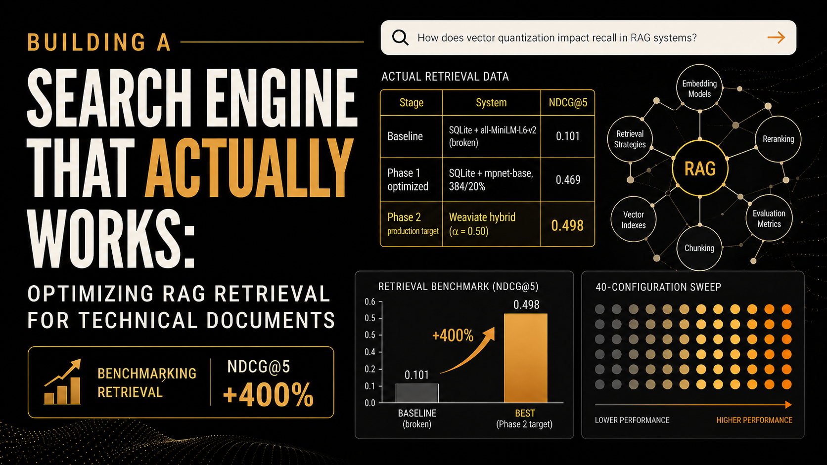
I started with a truly vibe coded system, where search quality baselined with a NDCG@5 of 0.101. By digging in and applying better understanding of search along with some scientific curiosity, I ended up with the optimized Weaviate hybrid at 0.498 — roughly a 400% improvement from start to finish. The baseline on my next system definitely won’t leave room for a 400% improvement, but I’ll still take the win this time.
| Stage | System | NDCG@5 |
|---|---|---|
| Baseline | SQLite + all-MiniLM-L6-v2 (broken) | 0.101 |
| Phase 1 optimized | SQLite + mpnet-base, 384/20% | 0.469 |
| Phase 2 production target | Weaviate hybrid (α=0.50) | 0.498 |
The migration to Weaviate hybrid is the next step: wiring the FastAPI search endpoint to the Weaviate adapter, with the SQLite system held in place as a rollback. The agentic pipeline built on top of this retrieval layer is a separate topic — one I’ll cover soon.
The most important lessons from this project weren’t a specific model choice or chunking strategy. They were that silent failures are the hardest to fix, and you can’t just do Leroy Jenkins style vibe code systems you actually want to rely on - put in the work and understand how to measure the systems before you build.
The baseline system returned results. It just never returned the right results - and without measurement, there was no way to know. Building the evaluation harness first, before changing anything, made every subsequent decision defensible. I’ll continue to test and refine this system, another topic that I’m yet to address is tabular data and photos. The system is currently incapable of returning a result for a search like “what does the fracture surface look like for low cycle fatigue failure in A356 aluminum?” and that’s something that would add significant value. But, the next step is integrating agentic retrieval with solid citation and traceability, look for that post in the coming weeks.