When One Data Point Costs $600 and Ten Weeks
What Machine Learning and Lean Six Sigma Can Teach Each Other About Scarce, Expensive Data
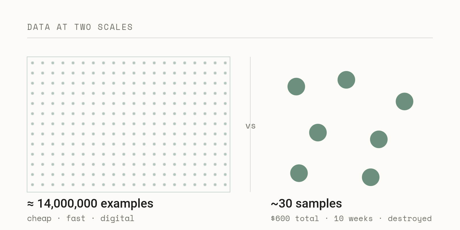
Producing a single set of tensile bars can cost upwards of $600, and the dollar figure is the cheap part. The real cost is time. Before you have a number to look at, you dial in color, select and tune molding parameters, cut purchase orders and wait on material, mold the parts, precondition them to a standard atmosphere or expose them to environmental conditions, pull them on a test frame, and finally analyze the data and write up the report. Ten weeks from “we should test this” to “here is the data” is routine, and for destructive environmental aging, where you are tracking how a coating or a sealant changes over simulated years, the timeline stretches further and every data point is a part you no longer have.
Now hold that next to how machine learning usually treats data. ImageNet, one of the datasets that kicked off the deep learning era, has roughly 14 million labeled images.[1] My characterization dataset for a new material might have thirty samples, and those thirty cost ten weeks and a stack of destroyed parts. As we start bolting AI tooling onto manufacturing and design, the gap between fourteen million and thirty is the thing nobody is really addressing. Closing it is not about a better model, it is about coupling the knowledge already inside the industry, the operators, technicians, and engineers who know how things actually get built, with the knowledge of the AI and ML engineers who know pipelines, evaluation harnesses, data integration, and LLM tooling. That pairing is where the real progress sits.
I am writing this from both sides of the fence, having spent fifteen years in materials, test labs, and quality systems and lately a lot of time building the AI tooling itself, and from where I sit the two communities are circling the same problem while barely talking to each other.
A Tale of Two Datasets
In a lot of machine learning, data is close to free: you scrape it, you log it, you buy it by the terabyte, and if a label is wrong you fix it and move on, because the marginal cost of one more example rounds to nothing. The physical world does not work that way, and the difference is not a detail, it changes what “doing data science” even means once you are working with parts instead of pixels.
When each observation costs real money and real weeks, you cannot brute-force your way to statistical power by collecting more, so you have to be deliberate about every single sample, which is a constraint the standard machine learning playbook, built on cheap and abundant data, mostly ignores. The manufacturing engineer and the data scientist are not really doing the same job even when they are both “working with data,” because one is optimizing over an ocean while the other is rationing drops, and almost everything downstream follows from that one difference.
The Traceability Gap
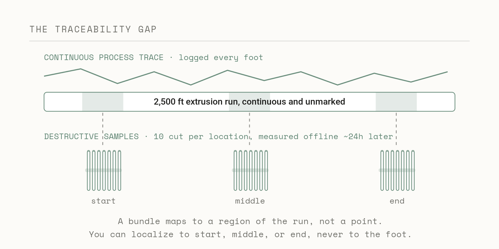
Here is the version of this problem that I never fully solved in a previous role. An extrusion line produces a 2,500-foot run of tubing, and the process is instrumented and continuous, so we log outer diameter, inner diameter, wall eccentricity, melt pressure, and barrel temperatures densely along the entire length, which gives us a rich and continuous record of how the line behaved. The trouble is that none of that record is physically stamped onto the product, because we are extruding a continuous length rather than discrete serialized parts, and there is no practical way to mark which foot of tubing was running when a given process excursion occurred. At least a day later the material gets cut down and samples are pulled for destructive tensile testing, and by then the link between a specific test result and the moment in the run that produced it is already gone.
This is the part the machine learning framing gets wrong if you are not careful, because the instinct is to call the continuous process parameters your features and the destructive tests your labels, then join them on a key and learn the mapping, except there is no key. You cannot take a tubing sample that had low tensile strength and walk it back to the eccentricity excursion or the pressure drift that caused it, because nobody recorded which physical location the sample came from – you’re relying on your ability to accurately measure the sample offline. So, in practice you end up using the two datasets separately, with the process trace telling you whether the line was stable, which you summarize as capability indices like Cpk, and the destructive samples telling you what the material properties were, measured fresh downstream, while relating one to the other stays educated guesswork about where in the run a problem most likely happened.
That matters because the clean feature-to-label join a lot of ML tooling assumes simply does not exist on a continuous process without deliberate effort to create it. The missing ingredient has a name on the manufacturing side, genealogy, meaning the traceable record of which material, which process conditions, and which moment produced a given piece, and without it the most basic question, “what was happening when this part was made,” has no answer. Building that genealogy back in is one of the highest-value and least glamorous things a data pipeline can do in a plant, and it turns out to be the key to learning anything over the long run.
Garbage In: Measurement and Sampling
Before you model anything, it is worth asking a question that is easy to skip when data feels abundant: how good is your ground truth, really? Manufacturing has a formal discipline for exactly this, Measurement System Analysis, and its workhorse is the Gage R&R study, which separates the variation that comes from the parts themselves from the variation introduced by the measurement system, meaning the gauge and the people operating it.[2] The criteria are blunt: if the measurement system accounts for more than 30% of the total observed variation it is unacceptable and has to be fixed before the numbers are trusted, while under 10% is considered good, so before you draw a single conclusion you prove that your ruler is actually a ruler.[2]
The closest machine learning analog is label noise, which is easy to leave unquantified. If two qualified annotators disagree on a label, or the same instrument returns a different reading on a re-measure, then part of what the model is straining to learn is just noise in the ground truth, and no amount of architecture search will rescue a measurement system that is 35% noise.
There is a second issue that maps less cleanly but matters just as much, and it is sampling bias. With samples this expensive you almost never get a clean random draw from the population, you get whatever was convenient, available, or cheap to test, and that quietly biases what the model learns. This is one of the places the influence runs the other direction, because interrogating how a sample was actually obtained is second nature to data scientists and statisticians, and it is a habit a plant that is used to testing whatever came off the line that afternoon would benefit from borrowing.
When the Process Won’t Hold Still
Process stability is its own kind of moving target, and the contrast between the two worlds is sharpest here. In machine learning, when the world drifts away from your training data you retrain the model or adjust parameters to track the new landscape, and while that is real work it is usually a matter of compute and time. In manufacturing a process shift can take your line down, delay shipments, and cost serious money, and “retraining” is rarely as simple as tweaking a parameter, because if the root cause is that you never accounted for seasonal environmental swings or a supply chain change, the fix might be re-cutting mold tooling, and production can sit offline for months while you do it.
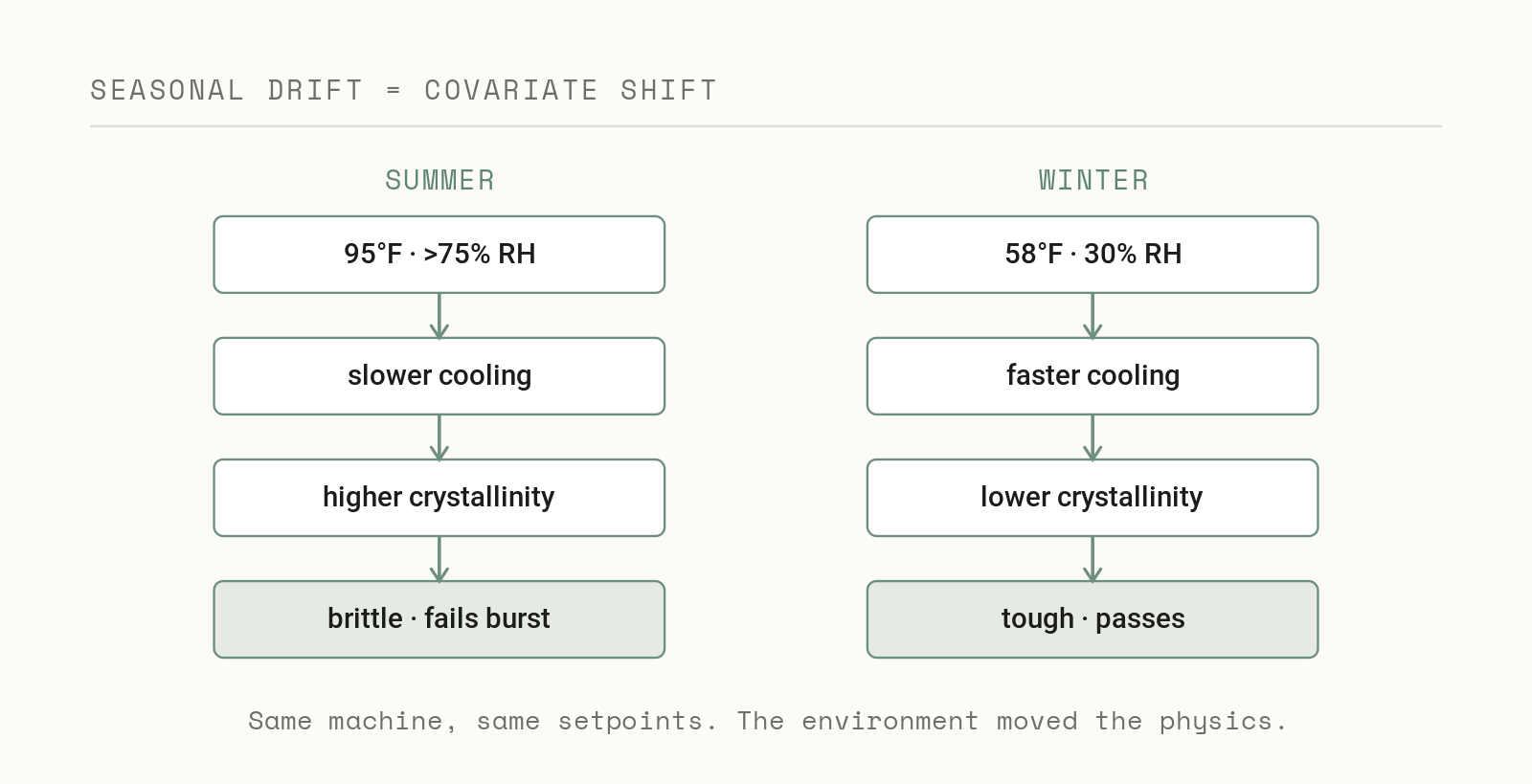
The operation that taught me this was an injection blow molding line running in an unconditioned facility in the Midwest, where in summer the shop floor sat around 95°F and frequently climbed past 75% relative humidity, and in winter it dropped to roughly 58°F and 30%. Final part performance was highly dependent on the degree of crystallinity in the polymer, which is directly tied to cooling, since for the particular polymer we were using, the longer a part took to cool the higher its crystallinity and the more brittle it became. Parts molded in January passed burst testing easily, while parts made in August off the same machine and at the same nominal settings came out extremely brittle, so it was the same program and the same setpoints producing different physics, entirely because the environment around the process was never controlled.
Machine learning has a precise name for what that does to any model built on the summer data, covariate shift, a form of dataset shift in which the distribution of the inputs changes between training and deployment while the underlying relationship holds.[3] The manufacturing engineer lives it as “the line behaves differently in August” and the ML engineer sees it as a silent accuracy drop in production, and it is the same phenomenon, except in the plant the cost of reacting to it is measured in scrap and downtime (or worse yet field failures) rather than GPU hours.
Predicting Before You Build
When every sample is expensive, the skill that matters most is learning as much as possible from as few experiments as possible, and manufacturing did not stumble into this, it built a formal science around it well before anyone used the phrase data science. Design of Experiments dates to Ronald Fisher in the 1920s and 1930s, whose factorial designs let you vary many factors at once and tease out their interactions rather than changing one variable at a time, and in the 1950s Box and Wilson added response surface methodology as a way to model and optimize a process with the fewest possible runs.[4] The whole purpose of DOE is to extract the most information per expensive experiment, which is the same problem that data-efficient machine learning works on today, arrived at decades earlier from the factory floor.
Six Sigma engineers have been doing data-efficient machine learning since the 1920s. They just called it Design of Experiments.
The design side widens this beyond the shop floor, which is part of why it matters. The familiar DMAIC cycle of Define, Measure, Analyze, Improve, and Control is for improving a process you already run and can collect data on, but when you are designing something new you often have no process data at all, and that is the domain of Design for Six Sigma, usually run as DMADV or IDOV, whose entire purpose is getting a design right before you build it.[5]
The signature tool there is Monte Carlo analysis, where instead of building parts and measuring whether an assembly holds tolerance, you describe each input dimension as a distribution, propagate thousands of simulated combinations through the transfer function that relates inputs to output, and read off the predicted distribution of the result, which lets you estimate yield and capability before a single part exists.[6] You are spending compute to avoid spending samples, and that is worth sitting with, because a simulation that predicts an output distribution from models of its inputs so you can decide before paying to build is conceptually the same move as using a surrogate model in machine learning, with both the Six Sigma engineer and the ML engineer substituting a cheap, validated approximation of reality for the expensive real thing.
Where the Two Worlds Converge
This comparison matters now because machine learning’s most active frontier is data efficiency, and it is converging on the same ideas, often from the same statistical roots. Active learning is the clearest case, since rather than labeling data blindly the model chooses the most informative examples to label next and reaches a target accuracy with far fewer labeled examples than labeling everything blindly would require, and if you have ever decided which sample to cut next based on where you expected to learn the most, you have done active learning by hand.[7] Bayesian optimization formalizes the same instinct, building a probabilistic model of the response and then choosing each next experiment to balance exploring the unknown against exploiting what already looks promising.[8]
I want to be careful not to overstate the relationship, because this is not machine learning independently reinventing Six Sigma in the dark, it is the same lineage. Bayesian optimization is openly described as an evolution of the design-of-experiments tradition, the adaptive successor to response surface methodology for high-dimensional, black-box problems, and Bayesian optimal experimental design traces back to Lindley in 1956.[9][10] Underneath the different vocabularies it really is all applied statistics, and ML did not replace experimental design so much as extend it to messier problems and wire it up to robots. That last part is literal in places, because Berkeley’s A-Lab paired language models trained on the literature with active learning grounded in thermodynamics and robotic synthesis to synthesize 36 new inorganic compounds from 57 targets in 17 days (the originally reported figure of 41 was revised down in a 2026 correction), running a closed loop of predict, build, measure, and update with minimal human intervention, which is in spirit a DMADV cycle executed by machines at a cadence no human lab could match.[11]
Here is something I’ve found useful, a map between the two worlds, with the plant on the left and the arXiv world on the right:
| Lean Six Sigma / industrial | Machine learning equivalent |
|---|---|
| Measurement System Analysis (Gage R&R) | Label noise and inter-annotator agreement |
| Design of Experiments (factorial, RSM) | Active learning, Bayesian optimization, optimal experimental design |
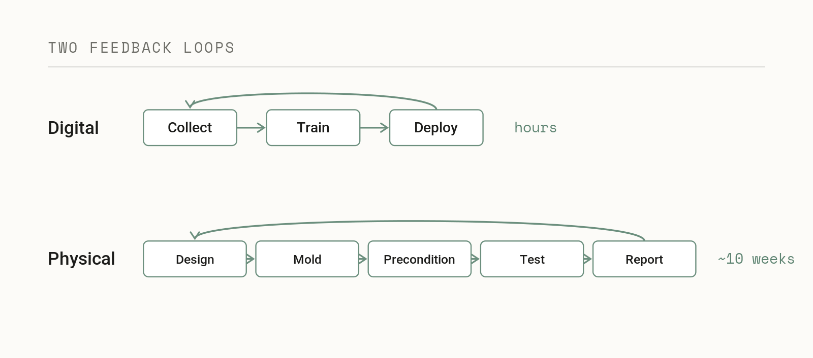
| DMAIC (improve an existing process) | The MLOps loop: train, deploy, monitor, retrain |
| DFSS / DMADV (design something new) | Cold-start modeling: transfer learning, informative priors, simulation |
| Monte Carlo tolerance analysis | Surrogate models and uncertainty propagation |
| Process capability (Cp/Cpk vs spec) | Model evaluation against acceptance thresholds |
| Continuous process params vs sampled output | Weak supervision and label scarcity (no key to join features to labels) |
| Seasonal ambient drift | Covariate shift, non-stationarity |
Read it from either side, because a quality engineer can see where their tools already live in the ML stack, and an ML engineer can see that the plant has battle-tested answers to problems the field is busy rediscovering.
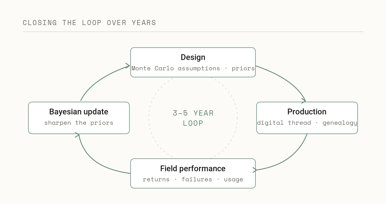
Closing the Loop Over Years
The hardest version of this problem is not a single experiment, it is the decade. The assumptions you bake into a Monte Carlo model or a qualification test are your best guess at design time, but the real distributions only reveal themselves once parts are in production and then in the field, and in many industries there are three to five years between designing something and having enough real-world data to know whether those assumptions held. The question that actually compounds value is how you carry a lesson from this year’s production runs and field returns back into the assumptions you will make on the next design, and most organizations have no reliable mechanism for it, so hard-won knowledge quietly evaporates between programs.
This is where the traceability gap from earlier comes back, because you cannot learn from a history you never recorded. The manufacturing answer is the digital thread, a continuous and traceable record that links design intent to production conditions to field performance and back again, establishing the genealogy of a part across its whole life instead of leaving design, the plant, and the field as disconnected islands.[12] Paired with a digital twin that is kept current as new data arrives, the thread turns “what was happening when this was made” into a question with an answer years after the fact, and it lets downstream reality feed back into the engineering decisions that started it all.[13]
The statistical machinery for actually using that history already exists, and it is Bayesian. Bayesian updating treats your original assumptions as a prior and revises them as field and test data accumulate, which is exactly the right shape for a multi-year loop, because the input distributions you guessed at for a tolerance analysis, or the life you assumed in an aging study, become priors that production and field data sharpen over time, so each new design starts from everything the last one taught rather than from a blank sheet.[14] Machine learning is reaching for the same capability under names like continual learning, the ambition being a system that keeps improving as new data arrives without being rebuilt from zero, and the plant and the lab want the identical thing: a way to make the next decision carry the weight of the entire history rather than just the last batch.
The Point
When data is expensive, the real constraint is experimental design, measurement rigor, and memory, not compute or algorithms, and the discipline for operating under that constraint already exists. Manufacturing spent a century building it, machine learning is now generalizing it with more powerful models and faster loops, and the two are unmistakably working the same problem from opposite ends.
There is a caveat worth stating plainly, because skipping it would be dishonest. Predicting before you build, and updating as you learn, only pays off if you stay honest about bias and uncertainty, since a surrogate model trained on thirty samples can be confidently wrong, a Monte Carlo result is only as good as the input distributions you assumed, and a Bayesian update inherits whatever bias lived in how the data was collected. The entire value of the Six Sigma toolkit is that it forces you to quantify uncertainty instead of waving it away, and that discipline matters more, not less, the moment you let a model stand in for an experiment.
So the version worth building is not an ML team parachuting in to disrupt the plant, and it is not the plant ignoring fifty years of progress in modeling. It is the operator and the engineer who know what the process actually does, working alongside the people who know how to build pipelines, evaluation harnesses, and the digital thread that ties it all together, with a shared goal of making the next decision carry the weight of everything the last one taught. The scarce, expensive data of the physical world is not a disadvantage to engineer around, it is the reason the rigor and the memory matter in the first place, and the teams that treat it that way are the ones who will close the gap between fourteen million and thirty.
References
[1] ImageNet. “ImageNet Dataset / ILSVRC.” en.wikipedia.org
[2] Automotive Industry Action Group (AIAG). “Measurement Systems Analysis (MSA) Reference Manual.” Summary of Gage R&R acceptance criteria. qimacros.com
[3] Quiñonero-Candela, J., Sugiyama, M., Schwaighofer, A., Lawrence, N. Dataset Shift in Machine Learning. MIT Press. mitpress.mit.edu
[4] American Society for Quality, “What Is Design of Experiments (DOE)?” and Penn State STAT 503, “A Quick History of DOE” (Fisher; Box & Wilson, RSM). asq.org · online.stat.psu.edu
[5] American Society for Quality. “Design for Six Sigma (DFSS)” (DMADV / IDOV). asq.org
[6] “Statistical Tolerancing using Monte Carlo Simulation.” Accendo Reliability. accendoreliability.com
[7] Settles, B. “Active Learning Literature Survey.” University of Wisconsin–Madison. burrsettles.com
[8] Shahriari, B., Swersky, K., Wang, Z., Adams, R. P., de Freitas, N. “Taking the Human Out of the Loop: A Review of Bayesian Optimization.” Proceedings of the IEEE, 2016. ieeexplore.ieee.org
[9] “Traditional or adaptive design of experiments? A pilot-scale comparison” (Bayesian optimization as an evolution of the DOE/RSM lineage). ScienceDirect. sciencedirect.com
[10] Lindley, D. V. (1956), on Bayesian optimal experimental design and expected information gain. See “Optimal experimental design: Formulations and computations,” Acta Numerica. cambridge.org
[11] Szymanski, N. J. et al. “An autonomous laboratory for the accelerated synthesis of inorganic materials.” Nature, 2023 (count corrected in 2026 to 36 of 57 targets). nature.com
[12] “Digital thread” (genealogy and lifecycle traceability connecting design, production, and field). en.wikipedia.org
[13] “Closing the Loop Between CAD, PLM, Digital Twins, and the Cloud.” Automation World (feeding field data back into design). automationworld.com
[14] Tian, et al. “Specifying prior distributions in reliability applications.” Applied Stochastic Models in Business and Industry, 2024 (Bayesian updating of priors with field/test data). onlinelibrary.wiley.com